#Formatting Time Using The Date Object and String Padding

[digital-marketing-29]

What is SQL and Data Types ?

SQL (Structured Query Language) uses various data types to define the kind of data that can be stored in a database. Each SQL database management system (DBMS) may have its own variations, but here are the most common SQL data types categorized broadly:

Numeric Data Types INT (or INTEGER) Description: Used to store whole numbers. The typical range is -2,147,483,648 to 2,147,483,647. Example: sql CREATE TABLE Employees ( EmployeeID INT PRIMARY KEY, Age INT );

INSERT INTO Employees (EmployeeID, Age) VALUES (1, 30), (2, 25);

SELECT * FROM Employees WHERE Age > 28; DECIMAL (or NUMERIC) Description: Fixed-point numbers with a defined precision and scale (e.g., DECIMAL(10, 2) allows 10 digits total, with 2 after the decimal). Example: sql CREATE TABLE Products ( ProductID INT PRIMARY KEY, Price DECIMAL(10, 2) );

INSERT INTO Products (ProductID, Price) VALUES (1, 19.99), (2, 5.50);

SELECT * FROM Products WHERE Price < 10.00;

Character Data Types CHAR(n) Description: Fixed-length character string. If the input string is shorter than n, it will be padded with spaces. Example: sql CREATE TABLE Users ( UserID INT PRIMARY KEY, Username CHAR(10) );

INSERT INTO Users (UserID, Username) VALUES (1, 'Alice '), (2, 'Bob ');

SELECT * FROM Users; VARCHAR(n) Description: Variable-length character string that can store up to n characters. It does not pad with spaces. Example: sql CREATE TABLE Comments ( CommentID INT PRIMARY KEY, CommentText VARCHAR(255) );

INSERT INTO Comments (CommentID, CommentText) VALUES (1, 'Great product!'), (2, 'Not what I expected.');

SELECT * FROM Comments WHERE CommentText LIKE '%great%'; TEXT Description: Used for storing large amounts of text. The maximum length varies by DBMS. Example: sql CREATE TABLE Articles ( ArticleID INT PRIMARY KEY, Content TEXT );

INSERT INTO Articles (ArticleID, Content) VALUES (1, 'This is a long article content…');

SELECT * FROM Articles WHERE ArticleID = 1;

Date and Time Data Types DATE Description: Stores date values in the format YYYY-MM-DD. Example: sql CREATE TABLE Orders ( OrderID INT PRIMARY KEY, OrderDate DATE );

INSERT INTO Orders (OrderID, OrderDate) VALUES (1, '2024-01-15'), (2, '2024-02-10');

SELECT * FROM Orders WHERE OrderDate > '2024-01-01'; DATETIME Description: Combines date and time into one type, typically formatted as YYYY-MM-DD HH:MM:SS. Example: sql CREATE TABLE Appointments ( AppointmentID INT PRIMARY KEY, AppointmentTime DATETIME );

INSERT INTO Appointments (AppointmentID, AppointmentTime) VALUES (1, '2024-01-15 14:30:00');

SELECT * FROM Appointments WHERE AppointmentTime < NOW();

Binary Data Types BLOB (Binary Large Object) Description: Used to store large binary data, such as images or files. Example: sql Copy code CREATE TABLE Images ( ImageID INT PRIMARY KEY, ImageData BLOB );

-- Assume we have binary data for an image to insert -- INSERT INTO Images (ImageID, ImageData) VALUES (1, ?);

Boolean Data Type BOOLEAN Description: Stores TRUE or FALSE values. In some systems, this might be represented as TINYINT (0 for FALSE, 1 for TRUE). Example: sql CREATE TABLE Subscriptions ( SubscriptionID INT PRIMARY KEY, IsActive BOOLEAN );

INSERT INTO Subscriptions (SubscriptionID, IsActive) VALUES (1, TRUE), (2, FALSE);

SELECT * FROM Subscriptions WHERE IsActive = TRUE;

JSON and XML Data Types JSON Description: Stores JSON-formatted data, allowing for flexible data structures. Example: sql CREATE TABLE Users ( UserID INT PRIMARY KEY, UserInfo JSON );

INSERT INTO Users (UserID, UserInfo) VALUES (1, '{"name": "Alice", "age": 30}');

SELECT * FROM Users WHERE UserInfo->>'name' = 'Alice'; XML Description: Used for storing XML data, allowing for structured data storage. Example: sql CREATE TABLE Configurations ( ConfigID INT PRIMARY KEY, ConfigData XML );

INSERT INTO Configurations (ConfigID, ConfigData) VALUES (1, 'dark');

SELECT * FROM Configurations WHERE ConfigData.exist('/config/setting[@name="theme" and text()="dark"]') = 1;

Special Data Types ENUM Description: A string object with a value chosen from a list of permitted values. Example: sql CREATE TABLE Products ( ProductID INT PRIMARY KEY, Size ENUM('Small', 'Medium', 'Large') );

INSERT INTO Products (ProductID, Size) VALUES (1, 'Medium'), (2, 'Large');

SELECT * FROM Products WHERE Size = 'Medium'; SET Description: A string object that can have zero or more values, each of which must be chosen from a predefined list. Example: sql CREATE TABLE UserRoles ( UserID INT, Roles SET('Admin', 'Editor', 'Viewer') );

INSERT INTO UserRoles (UserID, Roles) VALUES (1, 'Admin,Editor'), (2, 'Viewer');

SELECT * FROM UserRoles WHERE FIND_IN_SET('Admin', Roles);

[seldo]

Databases: how they work, and a brief history

My twitter-friend Simon had a simple question that contained much complexity: how do databases work?

Ok, so databases really confuse me, like how do databases even work?

— Simon Legg (@simonleggsays) November 18, 2019

I don't have a job at the moment, and I really love databases and also teaching things to web developers, so this was a perfect storm for me:

To what level of detail would you like an answer? I love databases.

— Laurie Voss (@seldo) November 18, 2019

The result was an absurdly long thread of 70+ tweets, in which I expounded on the workings and history of databases as used by modern web developers, and Simon chimed in on each tweet with further questions and requests for clarification. The result of this collaboration was a super fun tiny explanation of databases which many people said they liked, so here it is, lightly edited for clarity.

What is a database?

Let's start at the very most basic thing, the words we're using: a "database" literally just means "a structured collection of data". Almost anything meets this definition – an object in memory, an XML file, a list in HTML. It's super broad, so we call some radically different things "databases".

The thing people use all the time is, formally, a Database Management System, abbreviated to DBMS. This is a piece of software that handles access to the pile of data. Technically one DBMS can manage multiple databases (MySQL and postgres both do this) but often a DBMS will have just one database in it.

Because it's so frequent that the DBMS has one DB in it we often call a DBMS a "database". So part of the confusion around databases for people new to them is because we call so many things the same word! But it doesn't really matter, you can call an DBMS a "database" and everyone will know what you mean. MySQL, Redis, Postgres, RedShift, Oracle etc. are all DBMS.

So now we have a mental model of a "database", really a DBMS: it is a piece of software that manages access to a pile of structured data for you. DBMSes are often written in C or C++, but it can be any programming language; there are databases written in Erlang and JavaScript. One of the key differences between DBMSes is how they structure the data.

Relational databases

Relational databases, also called RDBMS, model data as a table, like you'd see in a spreadsheet. On disk this can be as simple as comma-separated values: one row per line, commas between columns, e.g. a classic example is a table of fruits:

apple,10,5.00 orange,5,6.50

The DBMS knows the first column is the name, the second is the number of fruits, the third is the price. Sometimes it will store that information in a different database! Sometimes the metadata about what the columns are will be in the database file itself. Because it knows about the columns, it can handle niceties for you: for example, the first column is a string, the second is an integer, the third is dollar values. It can use that to make sure it returns those columns to you correctly formatted, and it can also store numbers more efficiently than just strings of digits.

In reality a modern database is doing a whole bunch of far more clever optimizations than just comma separated values but it's a mental model of what's going on that works fine. The data all lives on disk, often as one big file, and the DBMS caches parts of it in memory for speed. Sometimes it has different files for the data and the metadata, or for indexes that make it easier to find things quickly, but we can safely ignore those details.

RDBMS are older, so they date from a time when memory was really expensive, so they usually optimize for keeping most things on disk and only put some stuff in memory. But they don't have to: some RDBMS keep everything in memory and never write to disk. That makes them much faster!

Is it still a database if all the structured data stays in memory? Sure. It's a pile of structured data. Nothing in that definition says a disk needs to be involved.

So what does the "relational" part of RDBMS mean? RDBMS have multiple tables of data, and they can relate different tables to each other. For instance, imagine a new table called "Farmers":

IDName 1bob 2susan

and we modify the Fruits table:

Farmer IDFruitQuantityPrice 1apple105.00 1orange56.50 2apple206.00 2orange14.75

.dbTable { border: 1px solid black; } .dbTable thead td { background-color: #eee; } .dbTable td { padding: 0.3em; }

The Farmers table gives each farmer a name and an ID. The Fruits table now has a column that gives the Farmer ID, so you can see which farmer has which fruit at which price.

Why's that helpful? Two reasons: space and time. Space because it reduces data duplication. Remember, these were invented when disks were expensive and slow! Storing the data this way lets you only list "susan" once no matter how many fruits she has. If she had a hundred kinds of fruit you'd be saving quite a lot of storage by not repeating her name over and over. The time reason comes in if you want to change Susan's name. If you repeated her name hundreds of times you would have to do a write to disk for each one (and writes were very slow at the time this was all designed). That would take a long time, plus there's a chance you could miss one somewhere and suddenly Susan would have two names and things would be confusing.

Relational databases make it easy to do certain kinds of queries. For instance, it's very efficient to find out how many fruits there are in total: you just add up all the numbers in the Quantity column in Fruits, and you never need to look at Farmers at all. It's efficient and because the DBMS knows where the data is you can say "give me the sum of the quantity colum" pretty simply in SQL, something like SELECT SUM(Quantity) FROM Fruits. The DBMS will do all the work.

NoSQL databases

So now let's look at the NoSQL databases. These were a much more recent invention, and the economics of computer hardware had changed: memory was a lot cheaper, disk space was absurdly cheap, processors were a lot faster, and programmers were very expensive. The designers of newer databases could make different trade-offs than the designers of RDBMS.

The first difference of NoSQL databases is that they mostly don't store things on disk, or do so only once in a while as a backup. This can be dangerous – if you lose power you can lose all your data – but often a backup from a few minutes or seconds ago is fine and the speed of memory is worth it. A database like Redis writes everything to disk every 200ms or so, which is hardly any time at all, while doing all the real work in memory.

A lot of the perceived performance advantages of "noSQL" databases is just because they keep everything in memory and memory is very fast and disks, even modern solid-state drives, are agonizingly slow by comparison. It's nothing to do with whether the database is relational or not-relational, and nothing at all to do with SQL.

But the other thing NoSQL database designers did was they abandoned the "relational" part of databases. Instead of the model of tables, they tended to model data as objects with keys. A good mental model of this is just JSON:

[ {"name":"bob"} {"name":"susan","age":55} ]

Again, just as a modern RDBMS is not really writing CSV files to disk but is doing wildly optimized stuff, a NoSQL database is not storing everything as a single giant JSON array in memory or disk, but you can mentally model it that way and you won't go far wrong. If I want the record for Bob I ask for ID 0, Susan is ID 1, etc..

One advantage here is that I don't need to plan in advance what I put in each record, I can just throw anything in there. It can be just a name, or a name and an age, or a gigantic object. With a relational DB you have to plan out columns in advance, and changing them later can be tricky and time-consuming.

Another advantage is that if I want to know everything about a farmer, it's all going to be there in one record: their name, their fruits, the prices, everything. In a relational DB that would be more complicated, because you'd have to query the farmers and fruits tables at the same time, a process called "joining" the tables. The SQL "JOIN" keyword is one way to do this.

One disadvantage of storing records as objects like this, formally called an "object store", is that if I want to know how many fruits there are in total, that's easy in an RDBMS but harder here. To sum the quantity of fruits, I have to retrieve each record, find the key for fruits, find all the fruits, find the key for quantity, and add these to a variable. The DBMS for the object store may have an API to do this for me if I've been consistent and made all the objects I stored look the same. But I don't have to do that, so there's a chance the quantities are stored in different places in different objects, making it quite annoying to get right. You often have to write code to do it.

But sometimes that's okay! Sometimes your app doesn't need to relate things across multiple records, it just wants all the data about a single key as fast as possible. Relational databases are best for the former, object stores the best for the latter, but both types can answer both types of questions.

Some of the optimizations I mentioned both types of DBMS use are to allow them to answer the kinds of questions they're otherwise bad at. RDBMS have "object" columns these days that let you store object-type things without adding and removing columns. Object stores frequently have "indexes" that you can set up to be able to find all the keys in a particular place so you can sum up things like Quantity or search for a specific Fruit name fast.

So what's the difference between an "object store" and a "noSQL" database? The first is a formal name for anything that stores structured data as objects (not tables). The second is... well, basically a marketing term. Let's digress into some tech history!

The self-defeating triumph of MySQL

Back in 1995, when the web boomed out of nowhere and suddenly everybody needed a database, databases were mostly commercial software, and expensive. To the rescue came MySQL, invented 1995, and Postgres, invented 1996. They were free! This was a radical idea and everybody adopted them, partly because nobody had any money back then – the whole idea of making money from websites was new and un-tested, there was no such thing as a multi-million dollar seed round. It was free or nothing.

The primary difference between PostgreSQL and MySQL was that Postgres was very good and had lots of features but was very hard to install on Windows (then, as now, the overwhelmingly most common development platform for web devs). MySQL did almost nothing but came with a super-easy installer for Windows. The result was MySQL completely ate Postgres' lunch for years in terms of market share.

Lots of database folks will dispute my assertion that the Windows installer is why MySQL won, or that MySQL won at all. But MySQL absolutely won, and it was because of the installer. MySQL became so popular it became synonymous with "database". You started any new web app by installing MySQL. Web hosting plans came with a MySQL database for free by default, and often no other databases were even available on cheaper hosts, which further accelerated MySQL's rise: defaults are powerful.

The result was people using mySQL for every fucking thing, even for things it was really bad at. For instance, because web devs move fast and change things they had to add new columns to tables all the time, and as I mentioned RDBMS are bad at that. People used MySQL to store uploaded image files, gigantic blobs of binary data that have no place in a DBMS of any kind.

People also ran into a lot of problems with RDBMS and MySQL in particular being optimized for saving memory and storing everything on disk. It made huge databases really slow, and meanwhile memory had got a lot cheaper. Putting tons of data in memory had become practical.

The rise of in-memory databases

The first software to really make use of how cheap memory had become was Memcache, released in 2003. You could run your ordinary RDBMS queries and just throw the results of frequent queries into Memcache, which stored them in memory so they were way, WAY faster to retrieve the second time. It was a revolution in performance, and it was an easy optimization to throw into your existing, RDBMS-based application.

By 2009 somebody realized that if you're just throwing everything in a cache anyway, why even bother having an RDBMS in the first place? Enter MongoDB and Redis, both released in 2009. To contrast themselves with the dominant "MySQL" they called themselves "NoSQL".

What's the difference between an in-memory cache like Memcache and an in-memory database like Redis or MongoDB? The answer is: basically nothing. Redis and Memcache are fundamentally almost identical, Redis just has much better mechanisms for retrieving and accessing the data in memory. A cache is a kind of DB, Memcache is a DBMS, it's just not as easy to do complex things with it as Redis.

Part of the reason Mongo and Redis called themselves NoSQL is because, well, they didn't support SQL. Relational databases let you use SQL to ask questions about relations across tables. Object stores just look up objects by their key most of the time, so the expressiveness of SQL is overkill. You can just make an API call like get(1) to get the record you want.

But this is where marketing became a problem. The NoSQL stores (being in memory) were a lot faster than the relational DBMS (which still mostly used disk). So people got the idea that SQL was the problem, that SQL was why RDBMS were slow. The name "NoSQL" didn't help! It sounded like getting rid of SQL was the point, rather than a side effect. But what most people liked about the NoSQL databases was the performance, and that was just because memory is faster than disk!

Of course, some people genuinely do hate SQL, and not having to use SQL was attractive to them. But if you've built applications of reasonable complexity on both an RDBMS and an object store you'll know that complicated queries are complicated whether you're using SQL or not. I have a lot of love for SQL.

If putting everything in memory makes your database faster, why can't you build an RDBMS that stores everything in memory? You can, and they exist! VoltDB is one example. They're nice! Also, MySQL and Postgres have kind of caught up to the idea that machines have lots more RAM now, so you can configure them to keep things mostly in memory too, so their default performance is a lot better and their performance after being tuned by an expert can be phenomenal.

So anything that's not a relational database is technically a "NoSQL" database. Most NoSQL databases are object stores but that's really just kind of a historical accident.

How does my app talk to a database?

Now we understand how a database works: it's software, running on a machine, managing data for you. How does your app talk to the database over a network and get answers to queries? Are all databases just a single machine?

The answer is: every DBMS, whether relational or object store, is a piece of software that runs on machine(s) that hold the data. There's massive variation: some run on 1 machine, some on clusters of 5-10, some run across thousands of separate machines all at once.

The DBMS software does the management of the data, in memory or on disk, and it presents an API that can be accessed locally, and also more importantly over the network. Sometimes this is a web API like you're used to, literally making GET and POST calls over HTTP to the database. For other databases, especially the older ones, it's a custom protocol.

Either way, you run a piece of software in your app, usually called a Client. That client knows the protocol for talking to the database, whether it's HTTP or WhateverDBProtocol. You tell it where the database server is on the network, it sends queries over and gets responses. Sometimes the queries are literally strings of text, like "SELECT * FROM Fruits", sometimes they are JSON payloads describing records, and any number of other variations.

As a starting point, you can think of the client running on your machine talking over the network to a database running on another machine. Sometimes your app is on dozens of machines, and the database is a single IP address with thousands of machines pretending to be one machine. But it works pretty much the same either way.

The way you tell your client "where" the DB is is your connection credentials, often expressed as a string like "http://username:password@mydb.com:1234" or "mongodb://...". But this is just a convenient shorthand. All your client really needs to talk to a database is the DNS name (like mydb.com) or an IP address (like 205.195.134.39), plus a port (1234). This tells the network which machine to send the query to, and what "door" to knock on when it gets there.

A little about ports: machines listen on specific ports for things, so if you send something to port 80, the machine knows the query is for your web server, but if you send it to port 1234, it knows the query is for your database. Who picks 1234 (In the case of Postgres, it's literally 5432)? There's no rhyme or reason to it. The developers pick a number that's easy to remember between 1 and 65,535 (the highest port number available) and hope that no other popular piece of software is already using it.

Usually you'll also have a username and password to connect to the database, because otherwise anybody who found your machine could connect to your database and get all the data in it. Forgetting that this is true is a really common source of security breaches!

There are bad people on the internet who literally just try every single IP in the world and send data to the default port for common databases and try to connect without a username or password to see if they can. If it works, they take all the data and then ransom it off. Yikes! Always make sure your database has a password.

Of course, sometimes you don't talk to your database over a network. Sometimes your app and your database live on the same machine. This is common in desktop software but very rare in web apps. If you've ever heard of a "database driver", the "driver" is the equivalent of the "client", but for talking to a local database instead of over a network.

Replication and scaling

Remember I said some databases run on just 1 machine, and some run on thousands of machines? That's known as replication. If you have more than one copy of a piece of data, you have a "replica" of that data, hence the name.

Back in the old days hardware was expensive so it was unusual to have replicas of your data running at the same time. It was expensive. Instead you'd back up your data to tape or something, and if the database went down because the hardware wore out or something, then you'd buy new hardware and (hopefully) reinstall your DBMS and restore the data in a few hours.

Web apps radically changed people's demands of databases. Before web apps, most databases weren't being continuously queried by the public, just a few experts inside normal working hours, and they would wait patiently if the database broke. With a web app you can't have minutes of downtime, far less hours, so replication went from being a rare feature of expensive databases to pretty much table stakes for every database. The initial form of replication was a "hot spare".

If you ran a hot spare, you'd have your main DBMS machine, which handled all queries, and a replica DBMS machine that would copy every single change that happened on the primary to itself. Primary was called m****r and the replica s***e because the latter did whatever the former told it to do, and at the time nobody considered how horrifying that analogy was. These days we call those things "primary/secondary" or "primary/replica" or for more complicated arrangements things like "root/branch/leaf".

Sometimes, people would think having a hot spare meant they didn't need a backup. This is a huge mistake! Remember, the replica copies every change in the main database. So if you accidentally run a command that deletes all the data in your primary database, it will automatically delete all the data in the replica too. Replicas are not backups, as the bookmarking site Magnolia famously learned.

People soon realized having a whole replica machine sitting around doing nothing was a waste, so to be more efficient they changed where traffic went: all the writes would go to the primary, which would copy everything to the replicas, and all the reads would go to the replicas. This was great for scale!

Instead of having 1 machine worth of performance (and you could swap to the hot spare if it failed, and still have 1 machine of performance with no downtime) suddenly you had X machines of performance, where X could be dozens or even hundreds. Very helpful!

But primary/secondary replication of this kind has two drawbacks. First, if a write has arrived at the primary database but not yet replicated to all the secondary machines (which can take half a second if the machines are far apart or overloaded) then somebody reading from the replica can get an answer that's out of date. This is known as a "consistency" failure, and we'll talk about it more later.

The second flaw with primary/second replication is if the primary fails, suddenly you can no longer write to your database. To restore the ability to do writes, you have to take one of the replicas and "promote" it to primary, and change all the other replicas to point at this new primary box. It's time-consuming and notoriously error-prone.

So newer databases invented different ways of arranging the machines, formally called "network topology". If you think of the way machines connect to each other as a diagram, the topology is the shape of that diagram. Primary/secondary looks like a star. Root/branch/leaf looks like a tree. But you can have a ring structure, or a mesh structure, or lots of others. A mesh structure is a lot of fun and very popular, so let's talk about more about them.

Mesh replication databases

In a mesh structure, every machine is talking to every other machine and they all have some portion of the data. You can send a write to any machine and it will either store it, or figure out what machine should store it and send it to that machine. Likewise, you can query any machine in the mesh, and it will give you the answer if it has the data, or forward your request to a machine that does. There's no "primary" machine to fail. Neat!

Because each machine can get away with storing only some of the data and not all of it, a mesh database can store much, much more data than a single machine could store. If 1 machine could store X data, then N machines could theoretically store N*X data. You can almost scale infinitely that way! It's very cool.

Of course, if each record only existed on one machine, then if that machine failed you'd lose those records. So usually in a mesh network more than one machine will have a copy of any individual record. That means you can lose machines without losing data or experiencing downtime; there are other copies lying around. In some mesh databases can also add a new machine to the mesh and the others will notice it and "rebalance" data, increasing the capacity of the database without any downtime. Super cool.

So a mesh topology is a lot more complicated but more resilient, and you can scale it without having to take the database down (usually). This is very nice, but can go horribly wrong if, for instance, there's a network error and suddenly half the machines can't see the other half of the machines in the mesh. This is called a "network partition" and it's a super common failure in large networks. Usually a partition will last only a couple of seconds but that's more than enough to fuck up a database. We'll talk about network partitions shortly.

One important question about a mesh DB is: how do you connect to it? Your client needs to know an IP address to connect to a database. Does it need to know the IP addresses of every machine in the mesh? And what happens when you add and remove machines from the mesh? Sounds messy.

Different Mesh DBs do it differently, but usually you get a load balancer, another machine that accepts all the incoming connections and works out which machine in the mesh should get the question and hands it off. Of course, this means the load balancer can fail, hosing your DB. So usually you'll do some kind of DNS/IP trickery where there are a handful of load balancers all responding on the same domain name or IP address.

The end result is your client magically just needs to know only one name or IP, and that IP always responds because the load balancer always sends you to a working machine.

CAP theory

This brings us neatly to a computer science term often used to talk about databases which is Consistency, Availability, and Partition tolerance, aka CAP or "CAP theory". The basic rule of CAP theory is: you can't have all 3 of Consistency, Availability and Partition Tolerance at the same time. Not because we're not smart enough to build a database that good, but because doing so violates physics.

Consistency means, formally: every query gets the correct, most up-to-date answer (or an error response saying you can't have it).

Availability means: every query gets an answer (but it's not guaranteed to be the correct one).

Partition Tolerance means: if the network craps out, the database will continue to work.

You can already see how these conflict! If you're 100% Available it means by definition you'll never give an error response, so sometimes the data will be out of date, i.e. not Consistent. If your database is Partition Tolerant, on the other hand, it keeps working even if machine A can't talk to machine B, and machine A might have a more recent write than B, so machine B will give stale (i.e. not Consistent) responses to keep working.

So let's think about how CAP theorem applies across the topologies we already talked about.

A single DB on a single machine is definitely Consistent (there's only one copy of the data) and Partition Tolerant (there's no network inside of it to crap out) but not Available because the machine itself can fail, e.g. the hardware could literally break or power could go out.

A primary DB with several replicas is Available (if one replica fails you can ask another) and Partition Tolerant (the replicas will respond even if they're not receiving writes from the primary) but not Consistent (because as mentioned earlier, the replicas might not have every primary write yet).

A mesh DB is extremely Available (all the nodes always answer) and Partition Tolerant (just try to knock it over! It's delightfully robust!) but can be extremely inconsistent because two different machines on the mesh could get a write to the same record at the same time and fight about which one is "correct".

This is the big disadvantage to mesh DBs, which otherwise are wonderful. Sometimes it's impossible to know which of two simultaneous writes is the "winner". There's no single authority, and Very Very Complicated Algorithms are deployed trying to prevent fights breaking out between machines in the mesh about this, with highly variable levels of success and gigantic levels of pain when they inevitably fail. You can't get all three of CAP and Consistency is what mesh networks lose.

In all databases, CAP isn't a set of switches where you are or aren't Consistent, Available, or Partition Tolerant. It's more like a set of sliders. Sliding up the Partition Tolerance generally slides down Consistency, sliding down Availability will give you more Consistency, etc etc.. Every DBMS picks some combination of CAP and picking the right database is often a matter of choosing what CAP combination is appropriate for your application.

Other topologies

Some other terms you frequently hear in the world of databases are "partitions" (which are different from the network partitions of CAP theorem) and "shards". These are both additional topologies available to somebody designing a database. Let's talk about shards first.

Imagine a primary with multiple replicas, but instead of each replica having all the data, each replica has a slice (or shard) of the data. You can slice the data lots of ways. If the database was people, you could have 26 shards, one with all names starting with A, one with all the names starting with B, etc..

Sharding can be helpful if the data is too big to all fit on one disk at a time. This is less of a problem than it used to be because virtual machines these days can effectively have infinity-sized hard drives.

The disadvantage of sharding is it's less Available: if you lose a shard, you lose everybody who starts with that letter! (Of course, your shards can also have replicas...) Plus your software needs to know where all the shards are and which one to ask a question. It's fiddly. Many of the problems of sharded databases are solved by using mesh topologies instead.

Partitions are another way of splitting up a database, but instead of splitting it across many machines, it splits the database across many files in a single machine. This is an old pattern that was useful when you had really powerful hardware and really slow disks, because you could install multiple disks into a single machine and put different partitions on each one, speeding up your achingly slow, disk-based database. These days there's not a lot of reason to use partitions of this kind.

Fin

That concludes this impromptu Databases 101 seminar! I hope you enjoyed learning a little bit more about this fantastically fun and critically important genre of software. from Seldo.Com Feed https://ift.tt/32XwZth

[qwertsypage]

D3.js Bar Chart Tutorial: Build Interactive JavaScript Charts and Graphs

Recently, we had the pleasure to participate in a machine learning project that involved libraries like React and D3.js. Among many tasks, I developed a few d3 bar charts and line charts that helped to process the result of ML models like Naive Bayes.

In this article, I would like to present my progress with D3.js so far and show the basic usage of this javascript chart library through the simple example of a bar chart.

After reading this article, you’ll learn how to create D3.js charts like this easily:

The full source code is available here.

We at RisingStack are fond of the JavaScript ecosystem, backend, and front-end development as well. Personally, I am interested in both of them. On the backend, I can see through the underlying business logic of an application while I also have the opportunity to create awesome looking stuff on the front-end. That’s where D3.js comes into the picture!

Update: a 2nd part of my d3.js tutorial series is available as well: Building a D3.js Calendar Heatmap (to visualize StackOverflow Usage Data)

What is D3.js?

D3.js is a data driven JavaScript library for manipulating DOM elements.

“D3 helps you bring data to life using HTML, SVG, and CSS. D3’s emphasis on web standards gives you the full capabilities of modern browsers without tying yourself to a proprietary framework, combining powerful visualization components and a data-driven approach to DOM manipulation.” - d3js.org

Why would You create charts with D3.js in the first place? Why not just display an image?

Well, charts are based on information coming from third-party resources which requires dynamic visualization during render time. Also, SVG is a very powerful tool which fits well to this application case.

Let’s take a detour to see what benefits we can get from using SVG.

The benefits of SVG

SVG stands for Scalable Vector Graphics which is technically an XML based markup language.

It is commonly used to draw vector graphics, specify lines and shapes or modify existing images. You can find the list of available elements here.

Pros:

Supported in all major browsers;

It has DOM interface, requires no third-party lib;

Scalable, it can maintain high resolution;

Reduced size compared to other image formats.

Cons:

It can only display two-dimensional images;

Long learning curve;

Render may take long with compute-intensive operations.

Despite its downsides, SVG is a great tool to display icons, logos, illustrations or in this case, charts.

Getting started with D3.js

I picked barcharts to get started because it represents a low complexity visual element while it teaches the basic application of D3.js itself. This should not deceive You, D3 provides a great set of tools to visualize data. Check out its github page for some really nice use cases!

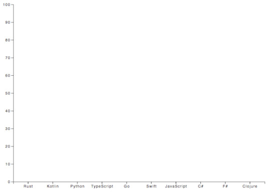
A bar chart can be horizontal or vertical based on its orientation. I will go with the vertical one in the form of a JavaScript Column chart.

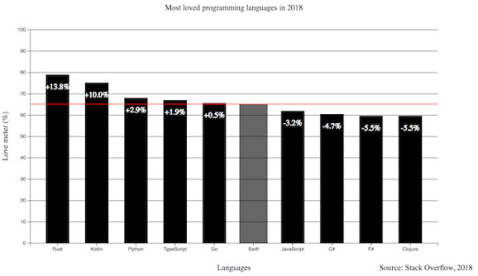
On this diagram, I am going to display the top 10 most loved programming languages based on Stack Overflow’s 2018 Developer Survey result.

How to draw bar graphs with SVG?

SVG has a coordinate system that starts from the top left corner (0;0). Positive x-axis goes to the right, while the positive y-axis heads to the bottom. Thus, the height of the SVG has to be taken into consideration when it comes to calculating the y coordinate of an element.

That’s enough background check, let’s write some code!

I want to create a chart with 1000 pixels width and 600 pixels height.

<body> <svg /> </body> <script> const margin = 60; const width = 1000 - 2 * margin; const height = 600 - 2 * margin; const svg = d3.select('svg'); </script>

In the code snippet above, I select the created <svg> element in the HTML file with d3 select. This selection method accepts all kind of selector strings and returns the first matching element. Use selectAll if You would like to get all of them.

I also define a margin value which gives a little extra padding to the chart. Padding can be applied with a <g> element translated by the desired value. From now on, I draw on this group to keep a healthy distance from any other contents of the page.

const chart = svg.append('g') .attr('transform', `translate(${margin}, ${margin})`);

Adding attributes to an element is as easy as calling the attr method. The method’s first parameter takes an attribute I want to apply to the selected DOM element. The second parameter is the value or a callback function that returns the value of it. The code above simply moves the start of the chart to the (60;60) position of the SVG.

Supported D3.js input formats

To start drawing, I need to define the data source I’m working from. For this tutorial, I use a plain JavaScript array which holds objects with the name of the languages and their percentage rates but it’s important to mention that D3.js supports multiple data formats.

The library has built-in functionality to load from XMLHttpRequest, .csv files, text files etc. Each of these sources may contain data that D3.js can use, the only important thing is to construct an array out of them. Note that, from version 5.0 the library uses promises instead of callbacks for loading data which is a non-backward compatible change.

Scaling, Axes

Let’s go on with the axes of the chart. In order to draw the y-axis, I need to set the lowest and the highest value limit which in this case are 0 and 100.

I’m working with percentages in this tutorial, but there are utility functions for data types other than numbers which I will explain later.

I have to split the height of the chart between these two values into equal parts. For this, I create something that is called a scaling function.

const yScale = d3.scaleLinear() .range([height, 0]) .domain([0, 100]);

Linear scale is the most commonly known scaling type. It converts a continuous input domain into a continuous output range. Notice the range and domain method. The first one takes the length that should be divided between the limits of the domain values.

Remember, the SVG coordinate system starts from the top left corner that’s why the range takes the height as the first parameter and not zero.

Creating an axis on the left is as simple as adding another group and calling d3’s axisLeft method with the scaling function as a parameter.

chart.append('g') .call(d3.axisLeft(yScale));

Now, continue with the x-axis.

const xScale = d3.scaleBand() .range([0, width]) .domain(sample.map((s) => s.language)) .padding(0.2) chart.append('g') .attr('transform', `translate(0, ${height})`) .call(d3.axisBottom(xScale));

Be aware that I use scaleBand for the x-axis which helps to split the range into bands and compute the coordinates and widths of the bars with additional padding.

D3.js is also capable of handling date type among many others. scaleTime is really similar to scaleLinear except the domain is here an array of dates.

Tutorial: Bar drawing in D3.js

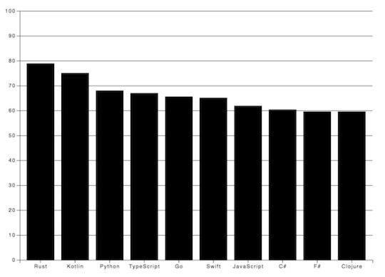
Think about what kind of input we need to draw the bars. They each represent a value which is illustrated with simple shapes, specifically rectangles. In the next code snippet, I append them to the created group element.

chart.selectAll() .data(goals) .enter() .append('rect') .attr('x', (s) => xScale(s.language)) .attr('y', (s) => yScale(s.value)) .attr('height', (s) => height - yScale(s.value)) .attr('width', xScale.bandwidth())

First, I selectAll elements on the chart which returns with an empty result set. Then, data function tells how many elements the DOM should be updated with based on the array length. enter identifies elements that are missing if the data input is longer than the selection. This returns a new selection representing the elements that need to be added. Usually, this is followed by an append which adds elements to the DOM.

Basically, I tell D3.js to append a rectangle for every member of the array.

Now, this only adds rectangles on top of each other which have no height or width. These two attributes have to be calculated and that’s where the scaling functions come handy again.

See, I add the coordinates of the rectangles with the attr call. The second parameter can be a callback which takes 3 parameters: the actual member of the input data, index of it and the whole input.

.attr(’x’, (actual, index, array) => xScale(actual.value))

The scaling function returns the coordinate for a given domain value. Calculating the coordinates are a piece of cake, the trick is with the height of the bar. The computed y coordinate has to be subtracted from the height of the chart to get the correct representation of the value as a column.

I define the width of the rectangles with the scaling function as well. scaleBand has a bandwidth function which returns the computed width for one element based on the set padding.

Nice job, but not so fancy, right?

To prevent our audience from eye bleeding, let’s add some info and improve the visuals! ;)

Tips on making javascript bar charts

There are some ground rules with bar charts that worth mentioning.

Avoid using 3D effects;

Order data points intuitively - alphabetically or sorted;

Keep distance between the bands;

Start y-axis at 0 and not with the lowest value;

Use consistent colors;

Add axis labels, title, source line.

D3.js Grid System

I want to highlight the values by adding grid lines in the background.

Go ahead, experiment with both vertical and horizontal lines but my advice is to display only one of them. Excessive lines can be distracting. This code snippet presents how to add both solutions.

chart.append('g') .attr('class', 'grid') .attr('transform', `translate(0, ${height})`) .call(d3.axisBottom() .scale(xScale) .tickSize(-height, 0, 0) .tickFormat('')) chart.append('g') .attr('class', 'grid') .call(d3.axisLeft() .scale(yScale) .tickSize(-width, 0, 0) .tickFormat(''))

I prefer the vertical grid lines in this case because they lead the eyes and keep the overall picture plain and simple.

Labels in D3.js

I also want to make the diagram more comprehensive by adding some textual guidance. Let’s give a name to the chart and add labels for the axes.

Texts are SVG elements that can be appended to the SVG or groups. They can be positioned with x and y coordinates while text alignment is done with the text-anchor attribute. To add the label itself, just call text method on the text element.

svg.append('text') .attr('x', -(height / 2) - margin) .attr('y', margin / 2.4) .attr('transform', 'rotate(-90)') .attr('text-anchor', 'middle') .text('Love meter (%)') svg.append('text') .attr('x', width / 2 + margin) .attr('y', 40) .attr('text-anchor', 'middle') .text('Most loved programming languages in 2018')

Interactivity with Javascript and D3

We got quite an informative chart but still, there are possibilities to transform it into an interactive bar chart!

In the next code block I show You how to add event listeners to SVG elements.

svgElement .on('mouseenter', function (actual, i) { d3.select(this).attr(‘opacity’, 0.5) }) .on('mouseleave’, function (actual, i) { d3.select(this).attr(‘opacity’, 1) })

Note that I use function expression instead of an arrow function because I access the element via this keyword.

I set the opacity of the selected SVG element to half of the original value on mouse hover and reset it when the cursor leaves the area.

You could also get the mouse coordinates with d3.mouse. It returns an array with the x and y coordinate. This way, displaying a tooltip at the tip of the cursor would be no problem at all.

Creating eye-popping diagrams is not an easy art form.

One might require the wisdom of graphic designers, UX researchers and other mighty creatures. In the following example I’m going to show a few possibilities to boost Your chart!

I have very similar values displayed on the chart so to highlight the divergences among the bar values, I set up an event listener for the mouseenter event. Every time the user hovers over a specific a column, a horizontal line is drawn on top of that bar. Furthermore, I also calculate the differences compared to the other bands and display it on the bars.

Pretty neat, huh? I also added the opacity example to this one and increased the width of the bar.

.on(‘mouseenter’, function (s, i) { d3.select(this) .transition() .duration(300) .attr('opacity', 0.6) .attr('x', (a) => xScale(a.language) - 5) .attr('width', xScale.bandwidth() + 10) chart.append('line') .attr('x1', 0) .attr('y1', y) .attr('x2', width) .attr('y2', y) .attr('stroke', 'red') // this is only part of the implementation, check the source code })

The transition method indicates that I want to animate changes to the DOM. Its interval is set with the duration function that takes milliseconds as arguments. This transition above fades the band color and broaden the width of the bar.

To draw an SVG line, I need a start and a destination point. This can be set via the x1, y1 and x2, y2 coordinates. The line will not be visible until I set the color of it with the stroke attribute.

I only revealed part of the mouseenter event here so keep in mind, You have to revert or remove the changes on the mouseout event. The full source code is available at the end of the article.

Let’s Add Some Style to the Chart!

Let’s see what we achieved so far and how can we shake up this chart with some style. You can add class attributes to SVG elements with the same attr function we used before.

The diagram has a nice set of functionality. Instead of a dull, static picture, it also reveals the divergences among the represented values on mouse hover. The title puts the chart into context and the labels help to identify the axes with the unit of measurement. I also add a new label to the bottom right corner to mark the input source.

The only thing left is to upgrade the colors and fonts!

Charts with dark background makes the bright colored bars look cool. I also applied the Open Sans font family to all the texts and set size and weight for the different labels.

Do You notice the line got dashed? It can be done by setting the stroke-width and stroke-dasharray attributes. With stroke-dasharray, You can define pattern of dashes and gaps that alter the outline of the shape.

line#limit { stroke: #FED966; stroke-width: 3; stroke-dasharray: 3 6; } .grid path { stroke-width: 3; } .grid .tick line { stroke: #9FAAAE; stroke-opacity: 0.2; }

Grid lines where it gets tricky. I have to apply stroke-width: 0 to path elements in the group to hide the frame of the diagram and I also reduce their visibility by setting the opacity of the lines.

All the other css rules cover the font sizes and colors which You can find in the source code.

Wrapping up our D3.js Bar Chart Tutorial

D3.js is an amazing library for DOM manipulation and for building javascript graphs and line charts. The depth of it hides countless hidden (actually not hidden, it is really well documented) treasures that waits for discovery. This writing covers only fragments of its toolset that help to create a not so mediocre bar chart.

Go on, explore it, use it and create spectacular JavaScript graphs & visualizations!

By the way, here's the link to the source code.

Have You created something cool with D3.js? Share with us! Drop a comment if You have any questions or would like another JavaScript chart tutorial!

Thanks for reading and see You next time when I'm building a calendar heatmap with d3.js!

D3.js Bar Chart Tutorial: Build Interactive JavaScript Charts and Graphs published first on https://koresolpage.tumblr.com/

[junker-town]

Dorktown: The quest for the six-win playoff team

Icon Sportswire via Getty Images

The NFC East is so bad that we’re in danger of seeing a six-win team in the playoffs. Maybe even a five-win team.

When the NFC East heads into Week 11, its leader will have three wins. THREE WINS! Ever since the NFL split into its eight-division format in 2002, there have been 152 opportunities for a team to drag its sorry three-win-having ass to Week 11 and find itself atop its division. This is the first and only time it has ever happened. Congratulations to the 3-5-1 Philadelphia Eagles.

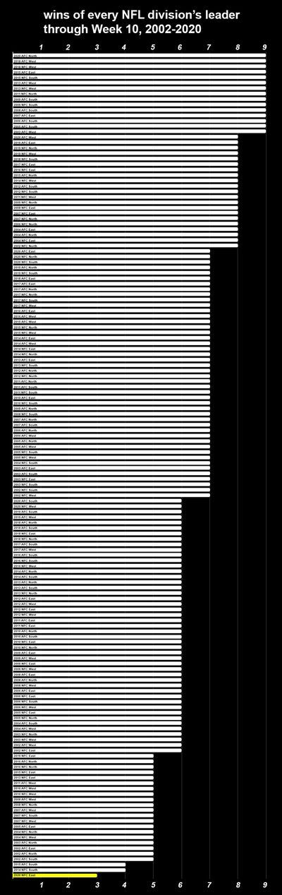
At this stage of the season, you almost always need at least six wins to lead a division, but the Eagles hold sole possession of first without even having to resort to tiebreakers:

Eagles (3-5-1)

Giants (3-7)

Washington (2-7)

Dallas (2-7)

Know this: throughout NFL history, no team has started 2-7 or 3-7 and made the postseason – unsurprising, since even if they’d somehow turned around and ran the table the rest of the way, 9-7 is often not good enough. This year, the NFC East is harboring three such teams, and all three are right in the thick of the playoff hunt.

If this were intentional, it would take a lot of orchestration. This is a two-stage rocket, and the first stage concerns the games these teams play against each other. Time and again, we’ve seen a not-great team vault into a record like 10-6 after proving just good enough to pick up cupcake wins within its weak division. That won’t work here. All four of these teams have to be more or less equally bad, such that they notch equal wins and losses against one another. So far, they’re doing a great job of this. These are their records within the division:

They’re sharing wins and losses as equally as the schedule allows; as of this date, the Giants and Cowboys are stuck with odd records only because they’ve played an odd number of division games. There’s every reason to hope that this equal winning and losing will continue: the Eagles have lost to Washington, who have lost to the Giants, who have lost to the Cowboys, who have lost to the Eagles, who have lost to the Giants, who have lost to the Cowboys, who have lost to Washington.

Now, the second stage of this rocket is a far more demanding one: these teams have to go out and lose to everyone else. And have they ever:

Look at all that orange. When NFC East teams are kicked out of the house by their exasperated parents and told to go play with the neighborhood children, they almost always lose. They’re 2-18-1 against the rest of the NFL this season. Let’s examine those three games that weren’t losses:

Eagles 25, 49ers 20. Philly squeaks by an injury-depleted Niners team that was missing their starting quarterback, their top two running backs, their starting center, star edge rushers Nick Bosa and Dee Ford, star cornerback Richard Sherman, and several other key guys. They did so after mounting a fourth-quarter comeback and barely surviving a last-minute drive led by their third-string quarterback.

Eagles 23, Bengals 23. Eagles quarterback Carson Wentz leads a last-minute drive to tie a Bengals team that is universally understood to be bad. Overtime goes like this: Bengals punt, Eagles punt, Bengals punt, Eagles punt, Bengals punt, Eagles punt, end of game. During their final two possessions, the Eagles make it well into Bengals territory before penalties pushed them back to their side of the field.

Cowboys 40, Falcons 39. Atlanta leads 39-24 with under six minutes left in the game. In one of the most spectacular comebacks I’ve ever seen in the NFL, Dak Prescott mounts three quick, heroic drives to pull out the squeaker. Of these three non-losses, this is the only particularly impressive one, although three things must be said about it. First, it hinged entirely on a recovered onside kick, which in today’s NFL counts as an incredible stroke of luck. Second, this happened against the Falcons. Not the Raheem Morris-coached Falcons who have really shown some fight over the last month, but the Dan Quinn Falcons who went 0-5. Third, Prescott was sadly lost to injury a few weeks later, robbing the NFC East of their only guy who’s proven himself capable of this kind of magic.

Two wins, 18 losses, one tie. Since ties are conventionally counted as 0.5 wins and 0.5 losses, this gives us a winning percentage of .119. Let’s flip that around: this season, teams who get to play an NFC East team this season have a winning percentage of .881. They’re juggernauts.

Consider how tough it is to find any split that will get you more favorable results than .881 over a span of at least 21 games. Let’s stack up a few splits that would seem favorable, with the help of Pro-Football-Reference’s Stathead tool.

Let’s have even more fun or even less fun, depending on who’s reading:

Brief aside: this is due to the sample size really thinning out toward the summit, but it is pretty funny that NFL teams’ winning percentages actually dip just slightly if they pass 42 points, and only recover once they hit 50. Similarly, that .881 winning percentage is based on a sample of just 21 games, so this chart wouldn’t quite hold up in an academic paper, but the fact remains: teams that score at least 30 points still have a less impressive winning percentage than literally any non-NFC East team that plays an NFC East team in 2020.

Now, it is true that the interdivisional schedules of these four teams have been pretty damn tough. Let’s use Football Outsiders’ DVOA rankings (through Week 9) to sort the quality of these teams from top to bottom, and count how many times our poor heroes have had to play them:

Rough stuff. Most of the time, they’ve run into good or very good teams. They’ve had to play the team with the NFL’s best record, the Steelers, three times (although it could just as easily be said that the Steelers have the NFL’s best record in part because they’ve gotten to play the NFC East three times).

Of course, the above chart omits the NFC East’s worst opponents: them. Come on out, fellas! There’s a bunch of folks here and they wanna laugh at you! Come on now!

This is why we can’t feel bad for any of these teams individually. Any tough opponents they’ve had to face elsewhere are more than balanced out by the privilege of being able to play their sorry selves.

You know, if I had the ability to assign teams to any division I wanted before the season started, with the objective of producing a division leader with as few wins as possible, I don’t know if I’d change anything. I think reality might have given us our best shot here, or at least something very, very close to it. If I just chose what I felt were the four very worst teams in the Jets, Bengals, Jags and Broncos, that could be trouble, because I suspect the Jets are miles worse than even the Bengals are. That would give the other three a punching bag that would allow them to pad their wins, which would blow the whole thing.

Instead, give me four teams who are both unmistakably bad, and almost the exact same degree of bad. Four teams who are dog shit in quadruplicate, and don’t appear to be much better or worse than each other in any material way.

So. Are we gonna see the NFL’s first-ever six-win playoff team? It’s absolutely in play, maybe even likely. I’m going to add a few more words in the hope of speaking them into existence:

We might see a five-win playoff team.

Let’s run through the remaining schedules of the Eagles, Giants, Cowboys and Football Team and see where we sit entering Week 11. Once again, we’ll rely on Football Outsiders’ DVOA.

Dallas Cowboys

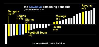
The Cowboys would need to win five of these seven games to reach seven wins and ruin our day. While they did play the Steelers close over the weekend, and they have four very winnable games ahead, this is a team that’s lost four straight. I just can’t see Andy Dalton coming back from the bye and winning five of seven.

(I’m not factoring home-field advantage here, although it’s worth noting that home teams only hold a slight advantage this season. The omnipresent NFC East loser vibes are far stronger in my view.)

Washington Football Team

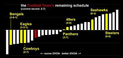
Same story as the Cowboys. Washington needs five wins to kill our dreams. I find the most useful way of framing this is: do we even trust them to get to three? I don’t.

New York Giants

The numbers are just slightly more friendly to the Giants: to make us unhappy, they need to win four of six, rather than five of seven. Their most likely path would be to beat the Cowboys and Bengals, then find some way to beat two 6-3 teams out of four.

I don’t see this as likely, but for purely unscientific reasons based on previous Giants team with entirely different rosters who stumbled backwards into sudden success, I think these guys are the most likely of the four to reach seven wins.

Especially because the Eagles’ upcoming schedule is so difficult.

Philadelphia Eagles

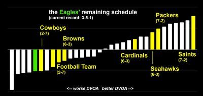
On paper, the Eagles have the easiest path to seven wins, as they only need to win four of their next seven. Four of these opponents are good-to-great (although the recent injury sustained by Drew Brees may mean beating the Saints is less unrealistic). The other three teams are subpar. All seven, though, hold a better DVOA than the Eagles.

The odds of Philadelphia reaching seven wins feel somewhere around 50-50 to me. I’ll take it! They still get to play two of their division rivals, and if they beat them both – which they’ll probably have to do in order to have a shot at 7-9 – that consequently deals a serious blow to all their seven-win aspirations, hopefully leaving the Eagles as the only team we’ll have left to worry about. From there, we hope that all five of the other teams, which are currently 6-3 or better, beat them.

Now, a five-win division champion? The road to that is tougher, but it’s absolutely possible. The math gets a little tricky, since in division games one team’s loss is another’s win, but you’re not at work here. You’re having fun. Simply scroll back up to those four charts and find:

four teams that can beat the Cowboys

four teams that can beat Washington

four teams that can beat the Giants

four teams that can beat the Eagles

If you can do that, you can imagine a team that lurches into the playoffs with a record of either 5-11 or 5-10-1. I need this. I need such a team to reach the playoffs while a very good team, like the Saints, Bucs, Cardinals, Rams or Seahawks, gets shut out of the postseason. Please, NFC East. Deliver us this future.

For further reading on the NFC East, check out this history lesson from Will, who points that these teams have been producing bad football since the 1930s.

[cristajha]

web designing and development overview

      Cascading style sheets Dropdowns, Cascading style sheet forms, CSS Rounded Corners by applying border-radius: 25px; that’s an excellent example of cascading style sheet rounded corners. Cascading style sheet Transitions, Cascading style sheet button, cascading style sheet templates.PHP Variables, PHP echo and print Statements, PHP Data Types, PHP Strings, PHP Constants, php operators, PHP if...else...elseif Statements, php scripting fundamentals, variables data types and expressions, operators in php, looping and conditional constructs, standard functions, arrays, user defined functions, error handling and reporting, php superglobals, php forms etc.

It is the work involved in developing a website for displaying on the internet. It is used for developing a static page toa  complex web page. It is mainly done or hired by professionals. Web development or website development is a part of information technology sector services. It is based on a content management system, there are three types of web development specialization front end developer back end developer and full stack developer. There are many tools of web development such as MySQL, Personal home page or hypertext preprocessor, hypertext markup language, wordpress etc.  

First of all let us discuss websites. A website is a collection of web pages. Usually designing means a preliminary sketch. Designing websites is called website designing.  Generally they are displayed or shown on the internet. It is an Information technology service which is given by any company or professional of that field. Mainly it contains or classified in three parts HTML5 which stands for hypertext markup language, CSS3 which stands for cascading style sheet, PHP which stands for hypertext preprocessor or personal home page, Bootstrap4, Javascript,jQuery and jQuery UI SQL which stands for structured query language, Web Hosting, Wordpress, AJAX which stands for  Asynchronous JavaScript And XML( extensible markup language), MySQL.  

1.Hypertext markup language: tim berners lee is the founder of hypertext markup language. It is a set of markup symbols or codes inserted into a file intended for display on the internet. First of all it is a computer language. By the help of hypertext mark up language we can create our own webpage. When we talk about hypertext markup language then here comes its content such as Hypertext markup language headings, hypertext markup language paragraph, hypertext markup language comments, hypertext markup language colors, hypertext markup language links, hypertext markup language images, hypertext markup language tables, hypertext markup language list which is of two types ordered list and unordered list. Hypertext markup language division,hypertext markup language id character which is described by # hash, hypertext markup language class for style, hypertext markup language forms, Hypertext markup language Canvas, hypertext markup language SVG. Look at below the format of hypertext markup language:

<!DOCTYPE html>

<html>

<head>

<style>

</style>

<title>

</title>

</head>

<body>

</body>

</html>

Let us discuss briefly:

1.The hypertext markup language Document Type: The declaration is not an HTML tag. It is an "information" to the browser about what document type to expect.

In HTML5, the <!DOCTYPE> declaration is simple:

<!DOCTYPE html>

2. The heading tag: The Hypertext markup language heading tags can be defined between h1 to h6. It is important to use the heading tag to show the heading structure. 

3. Style tag: The <style> tag is used to define style information (CSS) for a document. 

4.Title tag: a title tag described the main headline of the page. A title tag defines the title of the document. 

Body tag: a body tag defined the content of the page. It defined the subject matter of the web page.  such as headings, paragraphs, images, hyperlinks, tables, lists, etc.

  2. Cascading style sheet(CSS3): the invention of this language was done by Håkon Wium Lie on October 10, 1994. Cascading style sheet is a language which describes the style of a hypertext markup language document. It makes the website stylish, decorating and attractive. Its content are Cascading style sheet comment, cascading style sheet colors, Cascading style sheet background, cascading style sheet border, cascading style sheet text, cascading style sheet margins which is given outside the border, cascading style sheet font, cascading style sheet inside padding, cascading style sheet outline, cascading style sheet list which is ordered list and unordered list, Cascading style sheet height and width, cascading style sheet table, cascading style sheet fonts size, font color font family, cascading style sheet font awesome icon, Cascading style sheet styles three types are classified as below:

1.Inline cascading style sheet: a unique style to a single hypertext markup language element.let us take an example below:

<h1 style=”color: blue;”>This a web designing</h1>

2. Internal cascading style sheet: An internal CSS is used to define a style for a single HTML page.

An internal CSS is defined in the <head> section of an HTML page, within a <style> element:

<!DOCTYPE html>

<html>

<head>

<style>

body {background-color: powderblue;}

h1   {color: blue;}

p    {color: red;}

</style>

</head>

<body>

 <h1>This is a heading</h1>

<p>This is a paragraph.</p>

 </body>

</html>

   3. External cascading style sheet: With an external style sheet, you can change the look of an entire web site, by changing one file!

To use an external style sheet, add a link to it in the <head> section of the HTML page:

<!DOCTYPE html>

<html>

<head>

  <link rel="stylesheet" href="styles.css">

</head>

<body>

 <h1>This is a heading</h1>

<p>This is a paragraph.</p>

 </body>

</html>

Cascading style sheet links, cascading style sheet float, cascading style sheet alignment by using text-align:center; text-align:right; text-align: left; and text-align: justify; etc. Cascading style sheet opacity elements describe the transparency of the element. The opacity property can take a value from 0.0 - 1.0. The lower value, the more transparent:

  img{

Opacity: 0.5; 

}

Cascading style sheet navigation bars or menu bars are of two types: horizontal and vertical.

3. Pre hypertext processor or personal home page: it was invented by Rasmus Lerdorf in 1994. Pre Hypertext processor is a server scripting language, and a powerful tool for making dynamic and interactive web pages. The content of (core php)pre hypertext processor is pre hypertext processor installation.php comments are like below:

//this is a single line comment.

<?php =  it shows the starting tag.

?>   = it shows the ending tag.

/* this is knowns a multi line comment */

Advanced php content includes php date and time, php file upload, php cookies, php sessions, php object oriented programming language, MySQL Database,  Intro to PHP Components & Settings, http headers and output buffering, object and classes in php, inheritance and access modifiers, scope resolution operator, class constant parents self, static members and functions, final methods and final classes, abstract members and abstract classes, overview of directory and file processing, Functions Of File ComponentAuthentication in PHP,  File Uploads & Downloads,  Session & Cookie ManagementAuthentication in PHP,  PHP Functions for Managing Sessions.  PHP Functions for Managing Sessions.

Php with MySQL server content: intro to MySQL server, Overview of PHP MyAdmin Tool,  Database Creation,  MySQL Tables & Data Types, Database Connections,PHP functions specific to My SQL arrays, SQL statements and joins, all about record set, authentication in php, Ajax, Angular javascript, CMS(Content management system) overview.

4. Bootstrap4: Bootstrap is the most popular HTML, CSS, and JavaScript framework for developing responsive, mobile-first websites.Bootstrap Grid System Bootstrap's grid system allows up to 12 columns across the page.

If you do not want to use all 12 column individually, you can group the columns together to create wider columns: https://meashvitech.com

[htmlscraping-com]

Univocity-parsers - tutorial – uniVocity data integration

Welcome to univocity-parsers univocity-parsers is a collection of extremely fast and reliable Java-based parsers for CSV, TSV and Fixed Width files. It provides a consistent interface for handling different the different formats, and a solid framework for the development of new parsers. Introduction to univocity-parsers The project is developed and maintained by Univocity Software, an Australian company that develops custom data integration solutions using univocity, our commercial data integration framework, and the new univocity-html-parser for HTML scraping. While developing custom data migration services for our clients, involving a variety of text formats, we found that the parsers that currently exist for Java do not provide enough flexibility, throughput and reliability for massive and diverse (and messy) inputs. Another inconvenience is the difficulty in extending these parsers and dealing with a different beast for each format. We decided to then build our own architecture for parsing text files from the ground up. The main goal of this architecture is to provide maximum performance and flexibility while making it easy for anyone to create new parsers. univocity-parsers is currently used by many commercial and open-source projects, including Spark-CSV, Apache Camel and Apache Drill. Parsers univocity-parsers currently provides parsers for: CSV files - it’s the fastest and most flexible CSV parser for Java you can find Fixed-width files - it’s the fastest and most flexible Fixed-width (or fixed-length) parser for Java you can find TSV files - it’s the fastest and most flexible TSV parser for Java you can find Tutorial This library has MANY features so we split this tutorial in different sections. We suggest you to follow through this main tutorial to learn about the features shared among all parsers and then have a look at the specific sections for: Input files and methods All parsers work with an instance of java.io.Reader, java.io.File or java.io.InputStream. You will see calls such as getReader(“/examples/example.csv”) everywhere. This is just a helper method we use to build the examples (source code here): public Reader getReader(String relativePath) { … return new InputStreamReader(this.getClass().getResourceAsStream(relativePath), “UTF-8”); … } Writers on the other hand, can work instances of java.io.Writer, java.io.File or java.io.OutputStream. All parsers/writers have the exact same API and the code used to handle any format is almost the same. Differences are restricted to a few configuration options. In most of the examples, the files example.csv, example.tsv and example.txt file will be used as input for the different parsers provided by univocity-parsers. The information stored in each is exactly the same, only the format differs. This is the content in example.csv: # This example was extracted from Wikipedia (en.wikipedia.org/wiki/Comma-separated_values) # # 2 double quotes (“”) are used as the escape sequence for quoted fields, as per the RFC4180 standard # Year,Make,Model,Description,Price 1997,Ford,E350,“ac, abs, moon”,3000.00 1999,Chevy,“Venture ”“Extended Edition”“”,“”,4900.00 # Look, a multi line value. And blank rows around it! 1996,Jeep,Grand Cherokee,“MUST SELL! air, moon roof, loaded”,4799.00 1999,Chevy,“Venture ”“Extended Edition, Very Large”“”,,5000.00 ,,“Venture ”“Extended Edition”“”,“”,4900.00 The following example shows one of the many ways to parse all rows of this CSV file: CsvParserSettings settings = new CsvParserSettings(); //the file used in the example uses ’\n’ as the line separator sequence. //the line separator sequence is defined here to ensure systems such as MacOS and Windows //are able to process this file correctly (MacOS uses ’\r’; and Windows uses ’\r\n’). settings.getFormat().setLineSeparator(“\n”); // creates a CSV parser CsvParser parser = new CsvParser(settings); // parses all rows in one go. List<String[]> allRows = parser.parseAll(getReader(“/examples/example.csv”)); To parse all rows of a TSV, just switch to TsvParserSettings and TsvParser: TsvParserSettings settings = new TsvParserSettings(); settings.getFormat().setLineSeparator(“\n”); // creates a TSV parser TsvParser parser = new TsvParser(settings); // parses all rows in one go. List<String[]> allRows = parser.parseAll(getReader(“/examples/example.tsv”)); And to parse all rows of a Fixed-Width file, switch to FixedWidthParserSettings and FixedParser. Note this parser requires the additional configuration object FixedWidthFields to determine the width, alignment and padding of each field to parse: // creates the sequence of field lengths in the file to be parsed FixedWidthFields lengths = new FixedWidthFields(4, 5, 40, 40, 8); // creates the default settings for a fixed width parser FixedWidthParserSettings settings = new FixedWidthParserSettings(lengths); //sets the character used for padding unwritten spaces in the file settings.getFormat().setPadding(’_’); settings.getFormat().setLineSeparator(“\n”); // creates a fixed-width parser with the given settings FixedWidthParser parser = new FixedWidthParser(settings); // parses all rows in one go. List<String[]> allRows = parser.parseAll(getReader(“/examples/example.txt”)); The output of all examples above will be same: 1 [Year, Make, Model, Description, Price] ———————– 2 [1997, Ford, E350, ac, abs, moon, 3000.00] ———————– 3 [1999, Chevy, Venture “Extended Edition”, null, 4900.00] ———————– 4 [1996, Jeep, Grand Cherokee, MUST SELL! air, moon roof, loaded, 4799.00] ———————– 5 [1999, Chevy, Venture “Extended Edition, Very Large”, null, 5000.00] ———————– 6 [null, null, Venture “Extended Edition”, null, 4900.00] ———————– You can safely assume that any example provided in the following sections will work with any parser/writer. Settings and features that are specific to a format are discussed in dedicated, format-specific sections. So let’s get started! (very) Basic file parsing univocity-parsers comes with a basic API for parsing and processing data for all sorts of simpler use cases, which are demonstrated in this section, but the recommended (and faster) approach is Parsing with RowProcessors, a feature that puts univocity-parsers in another level of flexibility and power for handling the most intricate situations with almost no effort. For now, let’s start with the basics. Parsing all rows of a file in one go TsvParserSettings settings = new TsvParserSettings(); settings.getFormat().setLineSeparator(“\n”); // creates a TSV parser TsvParser parser = new TsvParser(settings); // parses all rows in one go. List<String[]> allRows = parser.parseAll(getReader(“/examples/example.tsv”)); You can also read all rows into Records, which allow you to convert rows to maps, fill existing maps, convert String values into other types such as int, float, Date and many more. Check the Using records section to learn more: // configure to grab headers from file. We want to use these names to get values from each record. settings.setHeaderExtractionEnabled(true); // creates a CSV parser CsvParser parser = new CsvParser(settings); // parses all records in one go. List<Record> allRecords = parser.parseAllRecords(getReader(“/examples/example.csv”)); for(Record record : allRecords){ print(“Year: ” + record.getValue(“year”, 2000)); //defaults year to 2000 if value is null. print(“, Model: ” + record.getString(“model”)); println(“, Price: ” + record.getBigDecimal(“price”)); } The output will be: Year: 1997, Model: E350, Price: 3000.00 Year: 1999, Model: Venture “Extended Edition”, Price: 4900.00 Year: 1996, Model: Grand Cherokee, Price: 4799.00 Year: 1999, Model: Venture “Extended Edition, Very Large”, Price: 5000.00 Year: 2000, Model: Venture “Extended Edition”, Price: 4900.00 To read all rows of a file (iterator-style) // creates a CSV parser CsvParser parser = new CsvParser(settings); // call beginParsing to read records one by one, iterator-style. parser.beginParsing(getReader(“/examples/example.csv”)); String[] row; while ((row = parser.parseNext()) != null) { println(out, Arrays.toString(row)); } // The resources are closed automatically when the end of the input is reached, // or when an error happens, but you can call stopParsing() at any time. // You only need to use this if you are not parsing the entire content. // But it doesn’t hurt if you call it anyway. parser.stopParsing(); For convenience, you can also use the parseNextRecord method, which will return an instance of Record instead of a raw String[]: // call beginParsing to read records one by one, iterator-style. parser.beginParsing(getReader(“/examples/example.csv”)); //among many other things, we can set default values of one ore more columns in the record metadata. //Let’s again set year to 2000 if it comes as null. parser.getRecordMetadata().setDefaultValueOfColumns(2000, “year”); Record record; while ((record = parser.parseNextRecord()) != null) { print(“Year: ” + record.getInt(“year”)); print(“, Model: ” + record.getString(“model”)); println(“, Price: ” + record.getBigDecimal(“price”)); } Using an actual iterator // creates a CSV parser CsvParser parser = new CsvParser(settings); for(String[] row : parser.iterate(getReader(“/examples/example.csv”))){ println(out, Arrays.toString(row)); } To iterate Records: for(Record record : parser.iterateRecords(getReader(“/examples/example.csv”))){ println(out, Arrays.toString(record.getValues())); } Parsing individual Strings If you are getting rows from an external source, and just need to parse each one, you can simply use the parseLine(String) method. The following example parses TSV lines: // creates a TSV parser TsvParser parser = new TsvParser(new TsvParserSettings()); String[] line; line = parser.parseLine(“A B C”); println(out, Arrays.toString(line)); line = parser.parseLine(“1 2 3 4”); println(out, Arrays.toString(line)); Which yields: [A, B, C] [1, 2, 3, 4] Column selection Parsing the entire content of each record in a file is a waste of CPU and memory when you are not interested in all columns. univocity-parsers lets you choose the columns you need, so values you don’t want are simply bypassed. The following examples can be found in the example class SettingsExamples: Consider the example.csv file with: Year,Make,Model,Description,Price 1997,Ford,E350,“ac, abs, moon”,3000.00 1999,Chevy,“Venture ”“Extended Edition”“”,“”,4900.00 … And the following selection: // Here we select only the columns “Price”, “Year” and “Make”. // The parser just skips the other fields parserSettings.selectFields(“Price”, “Year”, “Make”); // let’s parse with these settings and print the parsed rows. List<String[]> parsedRows = parseWithSettings(parserSettings); The output will be: 1 [3000.00, 1997, Ford] ———————– 2 [4900.00, 1999, Chevy] ———————– … The same output will be obtained with index-based selection. // Here we select only the columns by their indexes. // The parser just skips the values in other columns parserSettings.selectIndexes(4, 0, 1); // let’s parse with these settings and print the parsed rows. List<String[]> parsedRows = parseWithSettings(parserSettings); You can also opt to keep the original row format with all columns, but only the values you are interested in being processed: // Here we select only the columns “Price”, “Year” and “Make”. // The parser just skips the other fields parserSettings.selectFields(“Price”, “Year”, “Make”); // Column reordering is enabled by default. When you disable it, // all columns will be produced in the order they are defined in the file. // Fields that were not selected will be null, as they are not processed by the parser parserSettings.setColumnReorderingEnabled(false); // Let’s parse with these settings and print the parsed rows. List<String[]> parsedRows = parseWithSettings(parserSettings); Now the output will be: 1 [1997, Ford, null, null, 3000.00] ———————– 2 [1999, Chevy, null, null, 4900.00] ———————– 3 [1996, Jeep, null, null, 4799.00] … Settings Each parser has its own settings class, but many configuration options are common across all parsers. The following snippet demonstrates how to use each one of them: //You can configure the parser to automatically detect what line separator sequence is in the input parserSettings.setLineSeparatorDetectionEnabled(true); // sets what is the default value to use when the parsed value is null parserSettings.setNullValue(“<NULL>”); // sets what is the default value to use when the parsed value is empty parserSettings.setEmptyValue(“<EMPTY>”); // for CSV only // sets the headers of the parsed file. If the headers are set then ‘setHeaderExtractionEnabled(true)’ // will make the parser simply ignore the first input row. parserSettings.setHeaders(“a”, “b”, “c”, “d”, “e”); // prints the columns in reverse order. // NOTE: when fields are selected, all rows produced will have the exact same number of columns parserSettings.selectFields(“e”, “d”, “c”, “b”, “a”); // does not skip leading whitespaces parserSettings.setIgnoreLeadingWhitespaces(false); // does not skip trailing whitespaces parserSettings.setIgnoreTrailingWhitespaces(false); // reads a fixed number of records then stop and close any resources parserSettings.setNumberOfRecordsToRead(9); // does not skip empty lines parserSettings.setSkipEmptyLines(false); // sets the maximum number of characters to read in each column. // The default is 4096 characters. You need this to avoid OutOfMemoryErrors in case a file // does not have a valid format. In such cases the parser might just keep reading from the input // until its end or the memory is exhausted. This sets a limit which avoids unwanted JVM crashes. parserSettings.setMaxCharsPerColumn(100); // for the same reasons as above, this sets a hard limit on how many columns an input row can have. // The default is 512. parserSettings.setMaxColumns(10); // Sets the number of characters held by the parser’s buffer at any given time. parserSettings.setInputBufferSize(1000); // Disables the separate thread that loads the input buffer. By default, the input is going to be loaded incrementally // on a separate thread if the available processor number is greater than 1. Leave this enabled to get better performance // when parsing big files (> 100 Mb). parserSettings.setReadInputOnSeparateThread(false); // let’s parse with these settings and print the parsed rows. List<String[]> parsedRows = parseWithSettings(parserSettings); The output of the CSV parser with all these settings will be: 1 [<NULL>, <NULL>, <NULL>, <NULL>, <NULL>] ———————– 2 [Price, Description, Model, Make, Year] ———————– 3 [3000.00, ac, abs, moon, E350, Ford, 1997] ———————– 4 [4900.00, <EMPTY>, Venture “Extended Edition”, Chevy, 1999] ———————– 5 [<NULL>, <NULL>, <NULL>, <NULL>, ] ———————– 6 [<NULL>, <NULL>, <NULL>, <NULL>, ] ———————– 7 [4799.00, MUST SELL! air, moon roof, loaded, Grand Cherokee, Jeep, 1996] ———————– 8 [5000.00, <NULL>, Venture “Extended Edition, Very Large”, Chevy, 1999] ———————– 9 [4900.00, <EMPTY>, Venture “Extended Edition”, <NULL>, <NULL>] ———————– … Other settings skipBitsAsWhitespace: flag to configure the parser to consider BIT values 0 and 1 (effectively the ’\0’ and ’\1’ characters) as whitespace. Useful for processing database dumps that may export such values instead of the traditional '0’ and '1’’ characters. errorContentLength: in case of errors, limits the length of the problematic content that was parsed and is printed in error messages. Format Settings All parser settings have a default format definition. The following attributes are set by default for all parsers: lineSeparator (default System.getProperty(“line.separator”);): this is an array of 1 or 2 characters with the sequence that indicates the end of a line. Using this, you should be able to handle files produced by different operating systems. Of course, if you want your line separator to be “#$”, you can. normalizedNewline (default \n): used to represent the sequence of 2 characters used as a line separator (e.g. \r\n in Windows). It is used by our parsers/writers to easily handle portable line separators. When parsing, if the sequence of characters defined in lineSeparator is found while reading from the input, it will be transparently replaced by the normalizedNewline character. When writing, normalizedNewline is replaced by the lineSeparator sequence. comment (default #): if the first character of a line of text matches the comment character, then the row will be considered a comment and discarded from the input. Format-specific settings and features Each format has support for (hopefully) everything you will ever need and more. Check the sections dedicated to each one: Working with CSV Working with TSV Working with Fixed-Width Parsing with RowProcessors Everything you’ve seen so far is provided as a convenience for simpler situations, but univocity-parsers is built around the concept of RowProcessor and we encourage you to use them if you are after the best possible performance. The RowProcessor is a fairly simple interface with 3 methods: public interface RowProcessor { void processStarted(ParsingContext context); void rowProcessed(String[] row, ParsingContext context); void processEnded(ParsingContext context); } The settings object of all parsers come with a setProcessor method, which takes your RowProcessor implementation. When you are ready to parse the input, call parser.parse(), and each row parsed from the input will be sent to your processor’s rowProcessed method (that’s why parser.parse() is void). Before parsing the first row, processStarted will be called to notify you that rows are coming. After parsing the last row, or in the case of an error, all open resources will be closed and the process will stop. Once this completes the processEnded will be called so you can perform any additional housekeeping required. processEnded is guaranteed to run. All three methods have a ParsingContext object with some controls and information over the parsing process. The library provides many useful RowProcessor implementations by default and you can always provide your own. Most implementations of RowProcessor that come with the library by default come in two flavors: Abstract classes with one abstract method that delegates the result of each processed record to you, e.g. BeanProcessor, and ObjectRowProcessor Concrete classes with List in the name which indicates the the result of each processed record is added into a list. You can access the elements of this list once the processing has finished. e.g. BeanListProcessor, and ObjectRowListProcessor Introducing a few basic row processors The following example uses the RowListProcessor, which just stores the rows read from a file into a List: // The settings object provides many configuration options CsvParserSettings parserSettings = new CsvParserSettings(); //You can configure the parser to automatically detect what line separator sequence is in the input parserSettings.setLineSeparatorDetectionEnabled(true); // A RowListProcessor stores each parsed row in a List. RowListProcessor rowProcessor = new RowListProcessor(); // You can configure the parser to use a RowProcessor to process the values of each parsed row. // You will find more RowProcessors in the 'com.univocity.parsers.common.processor’ package, but you can also create your own. parserSettings.setProcessor(rowProcessor); // Let’s consider the first parsed row as the headers of each column in the file. parserSettings.setHeaderExtractionEnabled(true); // creates a parser instance with the given settings CsvParser parser = new CsvParser(parserSettings); // the 'parse’ method will parse the file and delegate each parsed row to the RowProcessor you defined parser.parse(getReader(“/examples/example.csv”)); // get the parsed records from the RowListProcessor here. // Note that different implementations of RowProcessor will provide different sets of functionalities. String[] headers = rowProcessor.getHeaders(); List<String[]> rows = rowProcessor.getRows(); Each row will contain: [Year, Make, Model, Description, Price] ======================= 1 [1997, Ford, E350, ac, abs, moon, 3000.00] ———————– 2 [1999, Chevy, Venture “Extended Edition”, null, 4900.00] ———————– 3 [1996, Jeep, Grand Cherokee, MUST SELL! air, moon roof, loaded, 4799.00] ———————– 4 [1999, Chevy, Venture “Extended Edition, Very Large”, null, 5000.00] ———————– 5 [null, null, Venture “Extended Edition”, null, 4900.00] ———————– You can also use a ObjectRowProcessor, which will produce rows of objects. You can convert values using an implementation of the Conversion interface. The Conversions class provides some useful defaults for you. For convenience, the ObjectRowListProcessor can be used to store all rows into a list. // ObjectRowProcessor converts the parsed values and gives you the resulting row. ObjectRowProcessor rowProcessor = new ObjectRowProcessor() { @Override public void rowProcessed(Object[] row, ParsingContext context) { //here is the row. Let’s just print it. println(out, Arrays.toString(row)); } }; // converts values in the “Price” column (index 4) to BigDecimal rowProcessor.convertIndexes(Conversions.toBigDecimal()).set(4); // converts the values in columns “Make, Model and Description” to lower case, and sets the value “chevy” to null. rowProcessor.convertFields(Conversions.toLowerCase(), Conversions.toNull(“chevy”)).set(“Make”, “Model”, “Description”); // converts the values at index 0 (year) to BigInteger. Nulls are converted to BigInteger.ZERO. rowProcessor.convertFields(new BigIntegerConversion(BigInteger.ZERO, “0”)).set(“year”); CsvParserSettings parserSettings = new CsvParserSettings(); parserSettings.getFormat().setLineSeparator(“\n”); parserSettings.setProcessor(rowProcessor); parserSettings.setHeaderExtractionEnabled(true); CsvParser parser = new CsvParser(parserSettings); //the rowProcessor will be executed here. parser.parse(getReader(“/examples/example.csv”)); After applying the conversions, the output will be: [1997, ford, e350, ac, abs, moon, 3000.00] [1999, null, venture “extended edition”, null, 4900.00] [1996, jeep, grand cherokee, must sell! air, moon roof, loaded, 4799.00] [1999, null, venture “extended edition, very large”, null, 5000.00] [0, null, venture “extended edition”, null, 4900.00] Using annotations to map your java beans Use the Parsed annotation to map the property to a field in the CSV file. You can map the property using a field name as declared in the headers, or the column index in the input. Each annotated operation maps to a Conversion and they are executed in the same sequence they are declared. This example works with the csv file bean_test.csv class TestBean { // if the value parsed in the quantity column is “?” or “-”, it will be replaced by null. @NullString(nulls = {“?”, “-”}) // if a value resolves to null, it will be converted to the String “0”. @Parsed(defaultNullRead = “0”) private Integer quantity; // The attribute type defines which conversion will be executed when processing the value. // In this case, IntegerConversion will be used. // The attribute name will be matched against the column header in the file automatically. @Trim @LowerCase // the value for the comments attribute is in the column at index 4 (0 is the first column, so this means fifth column in the file) @Parsed(index = 4) private String comments; // you can also explicitly give the name of a column in the file. @Parsed(field = “amount”) private BigDecimal amount; @Trim @LowerCase // values “no”, “n” and “null” will be converted to false; values “yes” and “y” will be converted to true @BooleanString(falseStrings = {“no”, “n”, “null”}, trueStrings = {“yes”, “y”}) @Parsed private Boolean pending; // Instances of annotated classes are created with by BeanProcessor and BeanListProcessor: // BeanListProcessor converts each parsed row to an instance of a given class, then stores each instance into a list. BeanListProcessor<TestBean> rowProcessor = new BeanListProcessor<TestBean>(TestBean.class); CsvParserSettings parserSettings = new CsvParserSettings(); parserSettings.getFormat().setLineSeparator(“\n”); parserSettings.setProcessor(rowProcessor); parserSettings.setHeaderExtractionEnabled(true); CsvParser parser = new CsvParser(parserSettings); parser.parse(getReader(“/examples/bean_test.csv”)); // The BeanListProcessor provides a list of objects extracted from the input. List<TestBean> beans = rowProcessor.getBeans(); Here is the output produced by the toString() method of each TestBean instance: [TestBean [quantity=1, comments=?, amount=555.999, pending=true], TestBean [quantity=0, comments=“ something ”, amount=null, pending=false]] The Headers annotation You can annotate a class with the Headers annotation to control what headers to use when parsing/writing, without having to provide any explicit configuration on the parser/writer settings: For example, consider the AnotherTestBean class: @Headers(sequence = {“pending”, “date”}, extract = true, write = true) public class AnotherTestBean { @Format(formats = {“dd-MMM-yyyy”, “yyyy-MM-dd”}, options = “locale=en”) @Parsed private Date date; @BooleanString(falseStrings = {“n”}, trueStrings = {“y”}) @Parsed private Boolean pending; // Let’s write a few instances of AnotherTestBean to an output: TsvWriterSettings settings = new TsvWriterSettings(); settings.setRowWriterProcessor(new BeanWriterProcessor<AnotherTestBean>(AnotherTestBean.class)); // We didn’t provide a java.io.Writer here, so all we can do is write to Strings (streaming) TsvWriter writer = new TsvWriter(settings); // Let’s write the headers declared in @Headers annotation of AnotherTestBean String headers = writer.writeHeadersToString(); // Now, let’s create an instance of our bean AnotherTestBean bean = new AnotherTestBean(); bean.setPending(true); bean.setDate(2012, Calendar.AUGUST, 5); // Calling processRecordToString will write the contents of the bean in a TSV formatted String String row1 = writer.processRecordToString(bean); // You can write whatever you need as well String row2 = writer.writeRowToString(“Random”, “Values”, “Here”); // Let’s change our bean and produce another String bean.setPending(false); String row3 = writer.processRecordToString(bean); This will write the following: pending date y 05-Aug-2012 Random Values Here n 05-Aug-2012 Error handling All sorts of errors can occur while processing data with a RowProcessor. You can get invalid values, unexpected formats, type errors, etc. In most cases you want to log these errors and continue processing your data. For that you can use a RowProcessorErrorHandler, which is a callback interface that will be used to report errors to you when they occur, with as much detail as possible: BeanListProcessor<AnotherTestBean> beanProcessor = new BeanListProcessor<AnotherTestBean>(AnotherTestBean.class); settings.setProcessor(beanProcessor); //Let’s set a RowProcessorErrorHandler to log the error. The parser will keep running. settings.setProcessorErrorHandler(new RowProcessorErrorHandler() { @Override public void handleError(DataProcessingException error, Object[] inputRow, ParsingContext context) { println(out, “Error processing row: ” + Arrays.toString(inputRow)); println(out, “Error details: column ’” + error.getColumnName() + “’ (index ” + error.getColumnIndex() + “) has value ’” + inputRow[error.getColumnIndex()] + “’”); } }); CsvParser parser = new CsvParser(settings); parser.parse(getReader(“/examples/bean_test.csv”)); println(out); println(out, “Printing beans that could be parsed”); println(out); for (AnotherTestBean bean : beanProcessor.getBeans()) { println(out, bean); //should print just one bean here } When running this example, you should get the following printed out: Error processing row: [yEs, 10-oct-2001] Error details: column 'pending’ (index 0) has value 'yEs’ Printing beans that could be parsed AnotherTestBean [date=10/Oct/2001, pending=false] Recovering from errors You can recover from errors using a RetryableErrorHandler: settings.setProcessorErrorHandler(new RetryableErrorHandler<ParsingContext>() { @Override public void handleError(DataProcessingException error, Object[] inputRow, ParsingContext context) { println(out, “Error processing row: ” + Arrays.toString(inputRow)); println(out, “Error details: column ’” + error.getColumnName() + “’ (index ” + error.getColumnIndex() + “) has value ’” + inputRow[error.getColumnIndex()] + “’. Setting it to null”); if(error.getColumnIndex() == 0){ setDefaultValue(null); } else { keepRecord(); //prevents the parser from discarding the row. } } }); Use keepRecord to prevent the parser from discarding your row. You can update the inputRow directly and at will then call keepRecord(). The setDefaultValue method assigns a default value to use in the column that could not be processed. Using this method will automatically instruct the parser to retry processing your row, so you don’t need to explicitly invoke keepRecord(). The output now should be: Error processing row: [yEs, 10-oct-2001] Error details: column 'pending’ (index 0) has value 'yEs’. Setting it to null Printing beans that could be parsed AnotherTestBean [date=10/Oct/2001, pending=null] AnotherTestBean [date=10/Oct/2001, pending=false] Collecting Comments If your input files have comments that might be useful for you to control the parsing process, you can configure the parser to collect them: // This configures the parser to store all comments found in the input. // You’ll be able to retrieve the last parsed comment or all comments parsed at // any given time during the parsing. settings.setCommentCollectionEnabled(true); CsvParser parser = new CsvParser(settings); parser.beginParsing(getReader(“/examples/example.csv”)); String[] row; while ((row = parser.parseNext()) != null) { // using the getContext method we have access to the parsing context, from where the comments found so far can be accessed // let’s get the last parsed comment and print it out in front of each parsed row. String comment = parser.getContext().lastComment(); if (comment == null || comment.trim().isEmpty()) { comment = “No relevant comments yet”; } println(“Comment: ” + comment + “. Parsed: ” + Arrays.toString(row)); } // We can also get all comments parsed. println(“\nAll comments found:\n——————-”); //The comments() method returns a map of line numbers associated with the comments found in them. Map<Long, String> comments = parser.getContext().comments(); for (Entry<Long, String> e : comments.entrySet()) { long line = e.getKey(); String commentAtLine = e.getValue(); println(“Line: ” + line + “: ’” + commentAtLine + “’”); } This should print the following to the output: Comment: 2 double quotes (“”) are used as the escape sequence for quoted fields, as per the RFC4180 standard. Parsed: [Year, Make, Model, Description, Price] Comment: 2 double quotes (“”) are used as the escape sequence for quoted fields, as per the RFC4180 standard. Parsed: [1997, Ford, E350, ac, abs, moon, 3000.00] Comment: 2 double quotes (“”) are used as the escape sequence for quoted fields, as per the RFC4180 standard. Parsed: [1999, Chevy, Venture “Extended Edition”, null, 4900.00] Comment: Look, a multi line value. And blank rows around it!. Parsed: [1996, Jeep, Grand Cherokee, MUST SELL! air, moon roof, loaded, 4799.00] Comment: Look, a multi line value. And blank rows around it!. Parsed: [1999, Chevy, Venture “Extended Edition, Very Large”, null, 5000.00] Comment: Look, a multi line value. And blank rows around it!. Parsed: [null, null, Venture “Extended Edition”, null, 4900.00] All comments found: ——————- Line: 0: 'This example was extracted from Wikipedia (en.wikipedia.org/wiki/Comma-separated_values)’ Line: 2: '2 double quotes (“”) are used as the escape sequence for quoted fields, as per the RFC4180 standard’ Line: 9: 'Look, a multi line value. And blank rows around it!’ Routines To make your life easier, we built a some pre-defined routines for handling common use cases, such as dumping data from a ResultSet, running parse-and-write operations, and more. Check the Routines section to learn more. Further Reading Feel free to proceed to the following sections (in any order). Bugs, contributions & support If you find a bug, please report it on github or send us an email on parsers@univocity.com. We try out best to eliminate all bugs as soon as possible and you’ll rarely see a bug open for more than 24 hours after it’s reported. We do our best to answer all questions. Enhancements/suggestions are implemented on a best effort basis. Fell free to submit your contribution via pull requests. Any little bit is appreciated, from improvements on documentation to a full blown rewrite from scratch. For commercial support, customizations or anything in between, please contact support@univocity.com. Thank you for using our parsers! The univocity team.

[myrtlecornish]

A Brief Tour of Swift UI

The best user interfaces are interactive and responsive to the user. UIKit is a capable framework that lets you build apps that users expect, but it can be tedious at time, not to mention having the flavor of an Objective-C toolkit.

SwiftUI takes advantage of Swift’s modern language features, giving us a modern framework that hits modern programming buzzwords.

It’s Declarative. Describe your UI in broad strokes using simple code.

It’s Compositional. You take existing views and connect them together and arrange them on the screen as you want.

It’s Automatic. Complex operations, like animations, can be done as a one-liner.

It’s Consistent. SwiftUI can be run on all of Apple’s platforms. It will take care to configure your UI (such as padding distance between on-screen controls, or dynamic type) so that it feels at home on whatever platform it’s running, whether it’s a Mac or the AppleTV.

Views and View Modifiers

Views are the heart of SwiftUI. According to Apple:

Views are defined declaratively as a function of their input

A View in SwiftUI is a struct that conforms to the View protocol. They are unrelated to UIViews (which are classes). A SwiftUI View is a value type, composed of the data that explains what you want to display.

Here’s a simple view:

struct Simpleiew : View { var body: some View { Text("I seem to be a verb") } }

Here SimpleView conforms to the View protocol. To appease the protocol, you need to provide a body, which is an opaque type. By using some new syntax, some View, we’re declaring that body is some kind of View, without having to specify a concrete type. Check out Swift Evolution Proposal 244 for more about opaque types.

The body is some View that describes what should be on the screen. In this case it’s a simple text label with a default configuration. Your body can be composed of multiple Views, such as a stack that arranges images horizontally.

Because body is a View, and it’s an opaque type, nobody really cares if a given View ends up being a single on-screen entity or a bunch of views composed in a stack or a list. This lets us compose complex hierarchies easily.

Chain Reaction

SwiftUI Views are value types, so we really don’t have stored properties to modify their look and feel. We need to declare our look and feel intentions to customize our views.

SwiftUI has ViewModifiers, such as .foreground to change the foreground color or .font to change a view’s font, that applies an attribute to a View. These modifiers also return the view they’re modifying, so you can chain them:

Text("SwiftUI is Great!") .foreground(.white) .padding() .background(Color.red)

This declarative syntax is very easy to read, letting you accomplish a lot with little code.

Stacks

You can build hierarchies of views. In UIKit, we use UIStackView to make vertical and horizontal stacks of UIViews. In SwiftUI, there’s an analogous HStack and VStack views that let you pile views horizontally or vertically.

This view positions one label above another.

VStack { Text("Swift UI is Great!") .foreground(.white) .padding() .background(Color.red) Text("I seem to be a verb") }

There’s also ZStack that lets you stack views on top of each other, like putting a label on top of an image.

You’re welcome to nest multiple stacks to compose complex view hierarchies. The stack views will automatically provide platform-appropriate defaults and if you don’t like the defaults, you can provide your own alignment and spacing.

Lists

SwiftUI lists look like tableviews in UIKit. In SwiftUI, the framework does the heavy lifting, freeing you from data source boilerplate.

Setting up a list with hard-coded views is really easy. Setting it up is exactly like setting up a stack:

struct ListView : View { var body: some View { List { Text("Look") Text("A") Text("TableView") } } }

The views inside the closure of a list serve as static cells.

The List also has an optional data parameter (that conforms to the Identifiable protocol) where you can provide some data to drive the creation of the cells inside the table.

Here’s a struct of a contact:

struct Contact: Identifiable { let id = UUID() let name: String }

Having a unique identifier in your identifiable data helps with list selection and cell manipulation.

And here’s a View that hardcodes a list of contacts:

struct ListView : View { let contacts = [Contact(name: "Arya"), Contact(name: "Bran"), Contact(name: "Jon"), Contact(name: "Sansa")] var body: some View { List(contacts) { contact in Text(contact.name) } } }

This is the magic bit:

List(contacts) { contact in Text(contact.name) }

This is telling the list: “for every Identifiable in this list of contacts, make a new Text view whose text contents are the contact’s name. You can add new folks to contacts, and the list will contain more rows.

State and Binding

Static hard-coded lists are great for initial prototyping of your ideas, but it’d be nice for the list to be dynamic, such as populating it with data from the internet. Or insert and delete new rows, and to rearrange things.

WWDC 2019 session 226 Data Flow Through SwiftUI tells us:

In SwiftUI data is a first class citizen

To manage state within our app, SwiftUI provides stateful binding to data and controls using property wrappers. Check out Swift Evolution Proposal 258 for more about property wrappers.

Here we’re using the the @State property wrapper to bind an isEnabled property to a toggle control:

struct EnabledTogglingView : View { @State private var isEnabled: Bool = false var body: some View { Toggle(isOn: $isEnabled) { Text("Enabled") } } }

Another quote from session 226, Data Flow Through SwiftUI:

SwiftUI manages the storage of any property you declare as a state. When the state value changes, the view invalidates its appearance and recomputes the body.

The state becomes the source of truth for a given view.

@State is great for prototyping, and for properties that are intrinsic to a view (such as this enabled state). To actually separate your data layer from your view layer, you need BindableObject.

So say we’re setting up a preference panel, or some kind of configuration panel with a sequence of toggle buttons. First, a model object for each individual setting:

class Settings: BindableObject { var didChange = PassthroughSubject<Bool, Never>() var isEnabled = false { didSet { didChange.send(self.isEnabled) } } }

Notice that Settings is a reference type (a class), which conforms to the BindableObject protocol. The PassthroughSubject doesn’t maintain any state - just passes through provided values. When a subscriber is connected and requests data, it will not receive any values until a .send() call is invoked.

struct BindableToggleView : View { @ObjectBinding var settings: Settings var body: some View { Toggle(isOn: $settings.isEnabled) { Text("Enabled") } } }

take another look at this line of code:

@ObjectBinding var settings: Settings

That’s weird. It’s not an optional then what’s it initialized to? Well, because settings is declared with the @ObjectBinding property wrapper, this tells the framework that it will be receiving data from some bindable object outside of the view. This object binding doesn’t need to be initialized.

You inject a BindableObject into the View that should use it. Here’s how our Settings gets hooked up to this BindableToggleView:

BindableToggleView(settings: Settings())

Your view does not care where the data lives or how it is populated disk, cache, network, osmosis. The view simply knows that it will be binding to some object when available.

The @ObjectBinding property wrapper creates a two-way binding. Whenever a mutation occurs the view automatically re-renders.

@ObjectBinding requires dependency injection to provide the data object. That can be inconvenient.

To make this object available anywhere within your app without dependency injection you can use the environment. New with SwiftUI you have an environment object that contains all kinds of information like screen size, orientation, locale, date format, etc. If you stick an object into the environment then that object can be accessed anywhere within your app. Think of it as a dictionary that is globally scoped within your app.

So how do you use it? The @EnvironmentObject property can help you with this.

struct BindableToggleView : View { @EnvironmentObject var settings: Settings var body: some View { Toggle(isOn: $settings.isEnabled) { Text("Enabled") } } }

In the above example, everything remains the same as seen previously, except you replace @ObjectBinding with @EnvironmentObject.

To inject an object into the environment you call the .environmentObject method.

ContentView().environmentObject(Settings())

An instance of Settings is now injected into the environment and is available to you anywhere within your app. When the object mutates then every view bound to it will receive the update and re-render its view. You no longer have to maintain a mental model of all the dependency-injections to keep your user interface in sync.

Animation

Animations in SwiftUI work like any view modifier. Basic animations can be achieved using the withAnimation method.

Here’s a View with two text labels:

struct ContentView: View { @State var scale: CGFloat = 1 var body: some View { VStack { Text("This text grows and shrinks") .scaleEffect(scale) Text("Scale it") .tapAction { self.scale = self.scale == 1.0 ? 5.0 : 1.0 } } } }

Tapping the second text label alters the size of the first text label, alternating its size between normal and five-times larger. The scaling happens instantly without any animation.

It’s a one-liner to make it animate smoothly.

Text("Scale it") .tapAction { withAnimation { self.scale = self.scale == 1.0 ? 5.0 : 1.0 } }

withAnimation can take an argument that lets you customize the animation. You can call it with a .basic animation, or you can have more fun with .spring animation that gives you control to make a beautiful spring effect.

Conclusion

SwiftUI is a delight to use. The focus is on creating an app because SwiftUI gets out of your way, taking care of a lot of annoying details. Design rich, interactive user interfaces by composing reusable views. Ensure data is coming into the system and not worry about keeping the view and model layers in sync. Finally, easily add animations to make views come alive.

A Brief Tour of Swift UI published first on https://johnellrod.weebly.com/